Analyzing Samples
Qiita now uses QIIME2 plugins for analysis.
Thanks to this, we’ve got new layout of the analysis panel and the following new features:
Alpha Diversity (including statistics calculations; example here)
Beta Diversity (including stats)
Principal Coordinate Analysis (PCoA), including ordination results and EMPeror plots (example here)
Taxa Summary (example here)
Creating A New Analysis
Create New Analysis Page
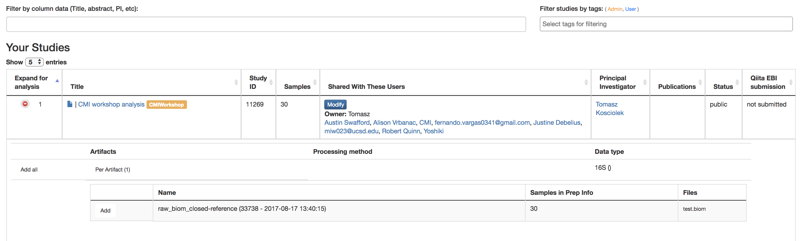
Filter results by column data (Title, Abstract, PI, etc.): Searches for studies with the title/abstract/PI/etc. that you inputted
Filter study by Study Tags: Searches for studies with the tag you searched for
Title: Brings you to Study Information Page of that experiment
Green Expand for Analysis Button: Reveals the studies done on this data that can be used for further analysis
Per Artifact Button: Reveals the names of the artifacts, the number of samples in the prep info, and the files
Add: Adds data to be analyzed
More than 1 can be done at once to do large meta-data analysis
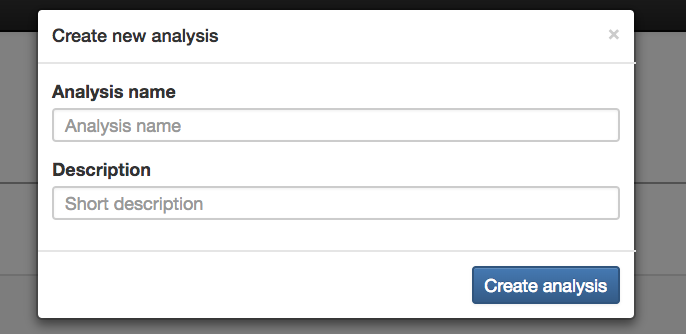
Create New Analysis: Creates the analysis using the data that has been added
Analysis Name (required): Name for the analysis that will be done
Description (optional): Description for the analysis that will be done
Single vs. Meta Analysis
Single analysis: One study chosen to analyze
Meta-analysis: Multiple studies chosen to analyze
You can only merge like data
Processing Network Page: Commands
Rarefying Features
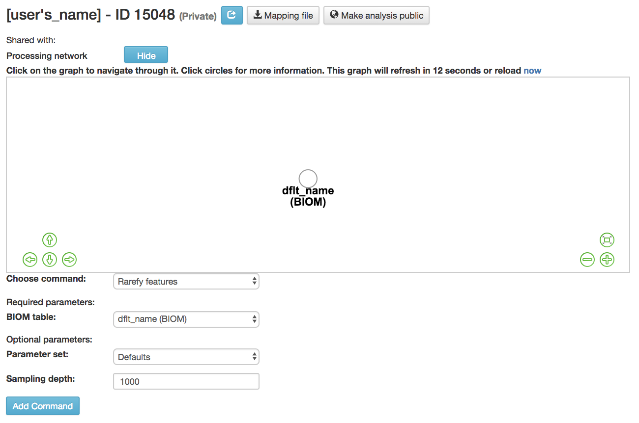
Rarefy features: Subsample frequencies from all samples without replacement so that the sum of frequencies in each sample is equal to the sampling-depth.
BIOM table (required): Feature table containing the samples for which features should be rarefied
Parameter set: Parameters at which the rarefication is run
Sampling depth (required): Total frequency that each sample should be rarefied to, samples where sum of frequencies is less than sampling depth will not be included in resulting table
Note that rarefaction has some advantages for beta-diversity analyses [11], but can have undesirable properties in tests of differential abundance [12]. To analyze your data with alternative normalization strategies, you can easily download the raw biom tables (see Downloading From Qiita) and load them into an analysis pipeline such as Phyloseq.
Filtering Samples by Metadata
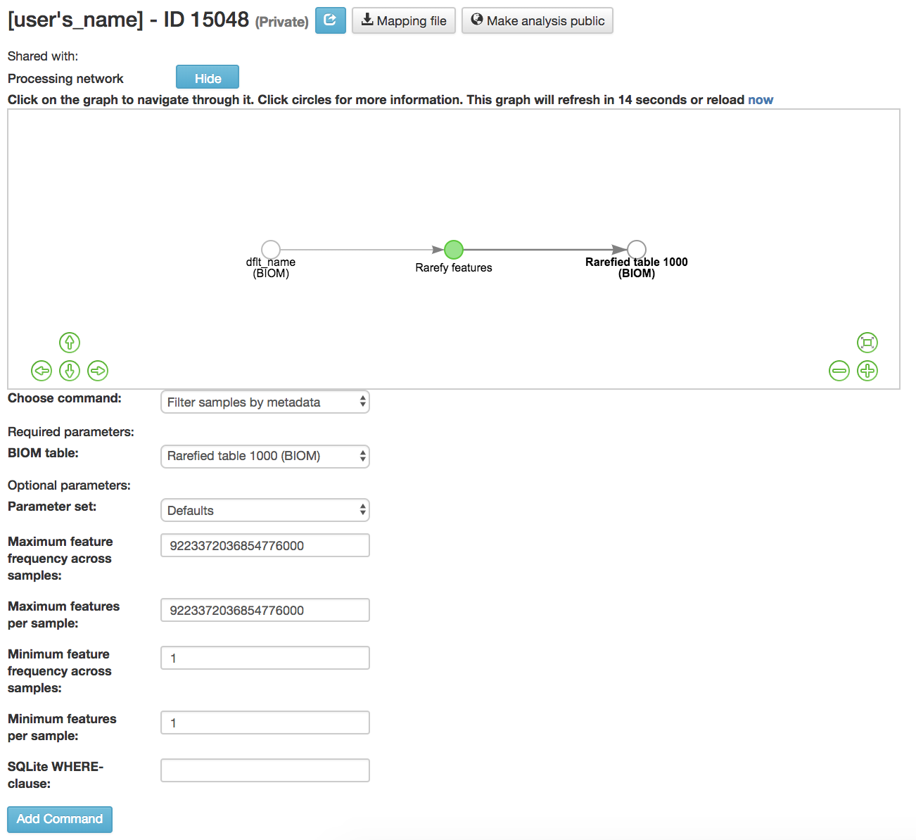
Filter samples by metadata: Filters samples from an OTU table on the basis of the number of observations in that sample, or on the basis of sample metadata
BIOM table (required): Feature table containing the samples for which features should be filtered
Maximum feature frequency across samples (optional): Maximum total frequency that a feature can have to be retained
Maximum features per sample (optional): Maximum number of features that a sample can have to be retained
Minimum feature frequency across samples (optional): Minimum total frequency that a feature must have to be retained
Minimum features per sample (optional): Minimum number of features that a sample can have to be retained
SQLite WHERE-clause (optional): Metadata group that is being filtered out
If you want to filter your samples by body_site and you want to only keep the tongue samples, fill the clause this way:
body_site = 'UBERON:tongue'If you want to filter your samples by body_site and you want to only remove the tongue samples, fill the clause this way:
body_site != 'UBERON:tongue'
Summarizing Taxa
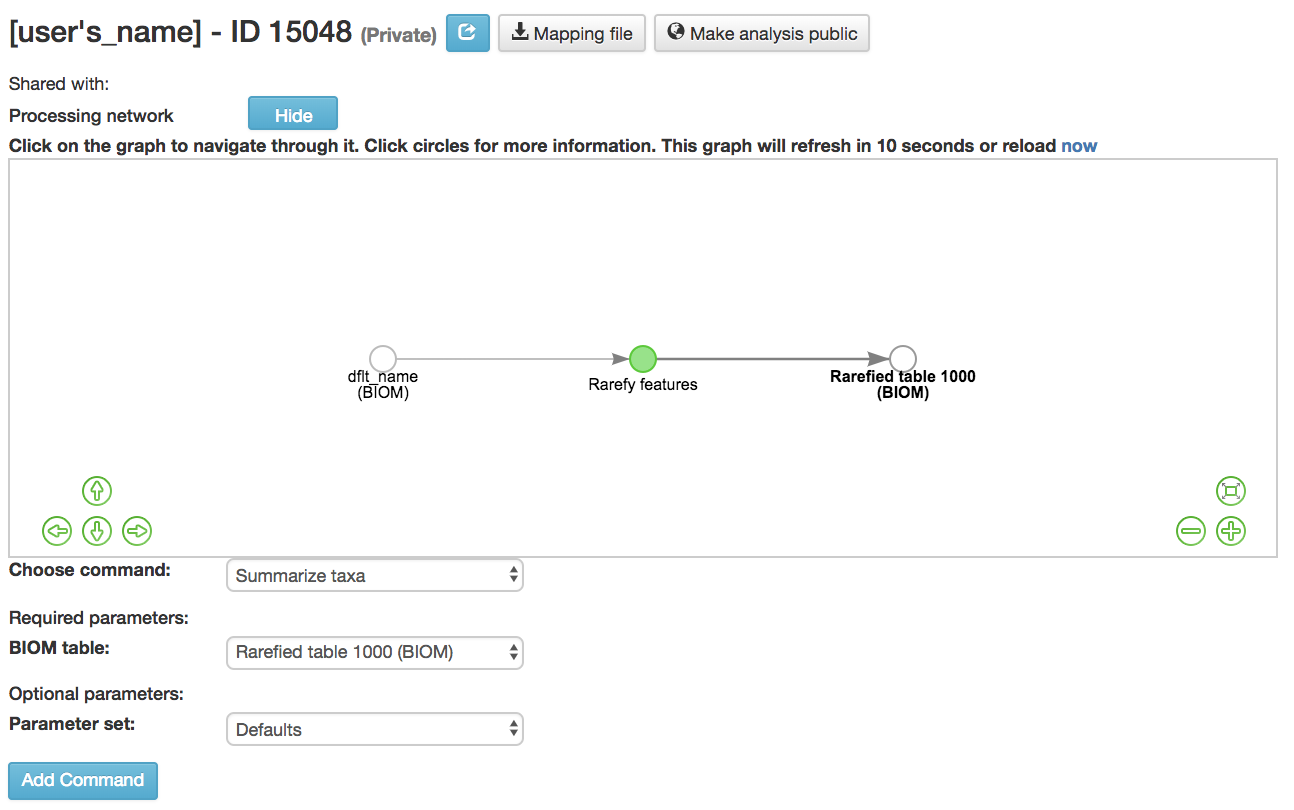
Summarize Taxa: Creates a bar plot of the taxa within the analysis
Can only be performed with closed-reference data
BIOM table (required): Feature table containing the samples to visualize at various taxonomic levels
Calculating Alpha Diversity
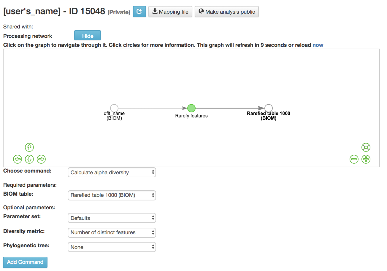
Calculate alpha diversity [13] : Measures the diversity within a sample
BIOM table (required): Feature table containing the samples for which alpha diversity should be computed
Diversity metric (required): Alpha diversity metric to be run
Abundance-based Coverage Estimator (ACE) metric [14] : Calculates the ACE metric
Estimates species richness using a correction factor
Berger-Parker Dominance Index [15] : Calculates Berger-Parker dominance index
Relative richness of the abundant species
Brillouin’s index [16] : Calculates Brillouin’s index
Measures the diversity of the species present
Use when randomness can’t be guaranteed
Chao1 index [14] : Calculates Chao1 index
Estimates diversity from abundant data
Estimates number of rare taxa missed from undersampling
Dominance measure: Calculates dominance measure
How equally the taxa are presented
Effective Number of Species (ENS)/Probability of intra-or interspecific encounter (PIE) metric [17] : Calculates Effective Number of Species (ENS)/Probability of intra-or interspecific encounter (PIE) metric
Shows how absolute amount of species, relative abundances of species, and their intraspecific clustering affect differences in biodiversity among communities
Faith’s phylogenetic diversity [18] : Calculates faith’s phylogenetic diversity
Measures of biodiversity that incorporates phylogenetic difference between species
Sum of length of branches
Fisher’s index [19] : Calculates Fisher’s index
Relationship between the number of species and the abundance of each species
Gini index [20] : Calculates Gini index
Measures species abundance
Assumes that the sampling is accurate and that additional data would fall on linear gradients between the values of the given data
Good’s coverage of counts [21] : Calculates Good’s coverage of counts.
Estimates the percent of an entire species that is represented in a sample
Heip’s evenness measure [22] : Calculates Heip’s evenness measure.
Removes dependency on species number
Lladser’s point estimate [23] : Calculates Lladser’ point estimate
Estimates how much of the environment contains unsampled taxa
Best estimate on a complete sample
Margalef’s richness index [24] : Calculates Margalef’s richness index
Measures species richness in a given area or community
Mcintosh dominance index D [25] : Calculates McIntosh dominance index D
Affected by the variation in dominant taxa and less affected by the variation in less abundant or rare taxa
Mcintosh evenness index E [22] : Calculates McIntosh’s evenness measure E
How evenly abundant taxa are
Menhinick’s richness index [24] : Calculates Menhinick’s richness index
The ratio of the number of taxa to the square root of the sample size
Michaelis-Menten fit to rarefaction curve of observed OTUs [26] : Calculates Michaelis-Menten fit to rarefaction curve of observed OTUs.
Estimated richness of species pools
Number of distinct features [27] : Calculates number of distinct OTUs
Number of double occurrences: Calculates number of double occurrence OTUs (doubletons)
OTUs that only occur twice
Number of single occurrences: Calculates number of single occurrence OTUs (singletons)
OTUs that appear only once in a given sample
Pielou’s evenness [28] : Calculates Pielou’s eveness
Measure of relative evenness of species richness
Robbins’ estimator [29] : Calculates Robbins’ estimator
Probability of unobserved outcomes
Shannon’s index [30] : Calculates Shannon’s index
Calculates richness and diversity using a natural logarithm
Accounts for both abundance and evenness of the taxa present
Simpson evenness measure E [31] : Calculates Simpson’s evenness measure E.
Diversity that account for the number of organisms and number of species
Simpson’s index [31] : Calculates Simpson’s index
Measures the relative abundance of the different species making up the sample richness
Strong’s dominance index (Dw) [32] : Calculates Strong’s dominance index
Measures species abundance unevenness
Phylogenetic tree (required for Faith PD): Phylogenetic tree to be used with alpha analyses (only include when necessary)
Currently the only tree that can be used is the GreenGenes 97% OTU based phylogenetic tree
Calculating Beta Diversity
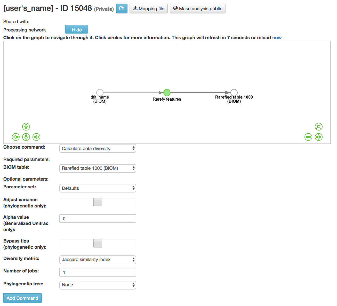
Calculate beta diversity [13] : Measured the diversity between samples
BIOM table (required): Feature table containing the samples for which beta diversity should be computed
Adjust variance [33] (phylogenetic only): Performs variance adjustment
Weighs distances based on the proportion of the relative abundance represented between the samples at a given node under evaluation
Alpha value (Generalized UniFrac only): Controls importance of sample proportions
1.0 is weighted normalized UniFrac. 0.0 is close to unweighted UniFrac, but only if the sample are dichotomized.
Bypass tips (phylogenetic only): In a bifurcating tree, the tips make up about 50% of the nodes in a tree. By ignoring them, specificity can be traded for reduced compute time. This has the effect of collapsing the phylogeny, and is analogous (in concept) to moving from 99% to 97% OTUs
Diversity metric (required): Beta diversity metric to be run
Bray-Curtis dissimilarity [34] : Calculates Bray–Curtis dissimilarity
Fraction of overabundant counts
Canberra distance [35] : Calculates Canberra distance
Overabundance on a feature by feature basis
Chebyshev distance [36] : Calculates Chebyshev distance
Maximum distance between two samples
City-block distance [37] : Calculates City-block distance
Similar to the Euclidean distance but the effect of a large difference in a single dimension is reduced
Correlation coefficient [38] : Measures Correlation coefficient
Measure of strength and direction of linear relationship between samples
Cosine Similarity [39] : Measures Cosine similarity
Ratio of the amount of common species in a sample to the mean of the two samples
Dice measures [40] : Calculates Dice measure
Statistic used for comparing the similarity of two samples
Only counts true positives once
Euclidean distance [41] : Measures Euclidean distance
Species-by-species distance matrix
Generalized Unifrac [42] : Measures Generalized UniFrac
Detects a wider range of biological changes compared to unweighted and weighted UniFrac
Hamming distance [43] : Measures Hamming distance
Minimum number of substitutions required to change one group to the other
Jaccard similarity index [44] : Calculates Jaccard similarity index
Fraction of unique features, regardless of abundance
Kulczynski dissimilarity index [45] : Measures Kulczynski dissimilarity index
Describes the dissimilarity between two samples
Matching components [46] : Measures Matching components
Compares indices under all possible situations
Rogers-tanimoto distance [47] : Measures Rogers-Tanimoto distance
Allows the possibility of two samples, which are quite different from each other, to both be similar to a third
Russel-Rao coefficient [48] : Calculates Russell-Rao coefficients
Equal weight is given to matches and non-matches
Sokal-Michener coefficient [49] : Measures Sokal-Michener coefficient
Proportion of matches between samples
Sokal-Sneath Index [50] : Calculates Sokal-Sneath index
Measure of species turnover
Species-by-species Euclidean [41] : Measures Species-by-species Euclidean
Standardized Euclidean distance between two groups
Each coordinate difference between observations is scaled by dividing by the corresponding element of the standard deviation
Squared Euclidean [41] : Measures squared Euclidean distance
Place progressively greater weight on samples that are farther apart
Unweighted Unifrac [51] : Measures unweighted UniFrac
Measures the fraction of unique branch length
Weighted Minkowski metric [52] : Measures Weighted Minkowski metric
Allows the use of the k-means-type paradigm to cluster large data sets
Weighted normalized UniFrac [53] : Measures Weighted normalized UniFrac
Takes into account abundance
Normalization adjusts for varying root-to-tip distances.
Weighted unnormalized UniFrac [53] : Measures Weighted unnormalized UniFrac
Takes into account abundance
Doesn’t correct for unequal sampling effort or different evolutionary rates between taxa
Yule index [19] : Measures Yule index
Measures biodiversity
Determined by the diversity of species and the proportions between the abundance of those species.
Number of jobs: Number of workers to use
Phylogenetic tree (required for Weighted Minkowski metric and all UniFrac metrics): Phylogenetic tree to be used with beta analyses (only include when necessary)
Currently the only tree that can be used is the GreenGenes 97% OTU based phylogenetic tree
Calculating Alpha Correlation
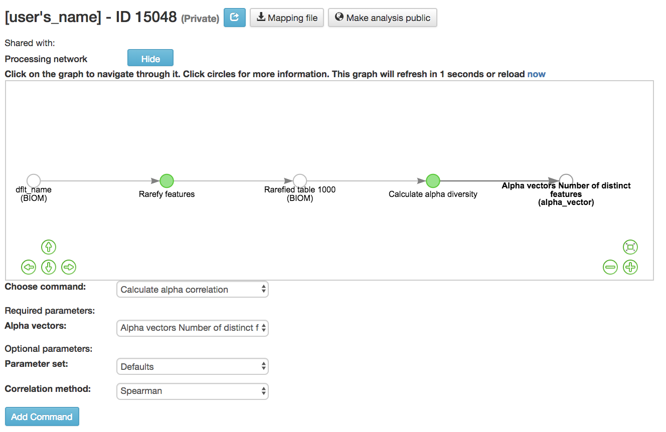
Calculate alpha correlation [54] : Determines if the numeric sample metadata category is correlated with alpha diversity
Performing Principal Coordinate Analysis
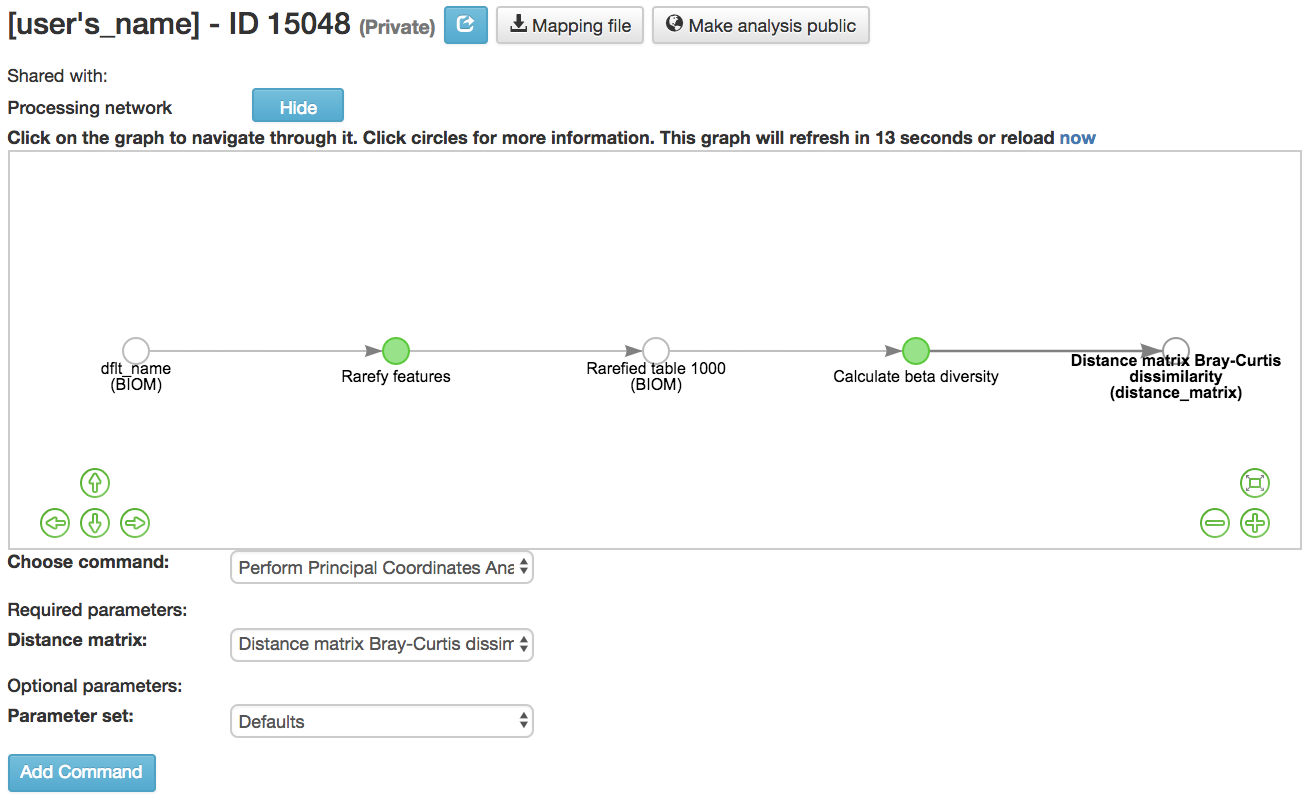
Calculating Beta Group Significance
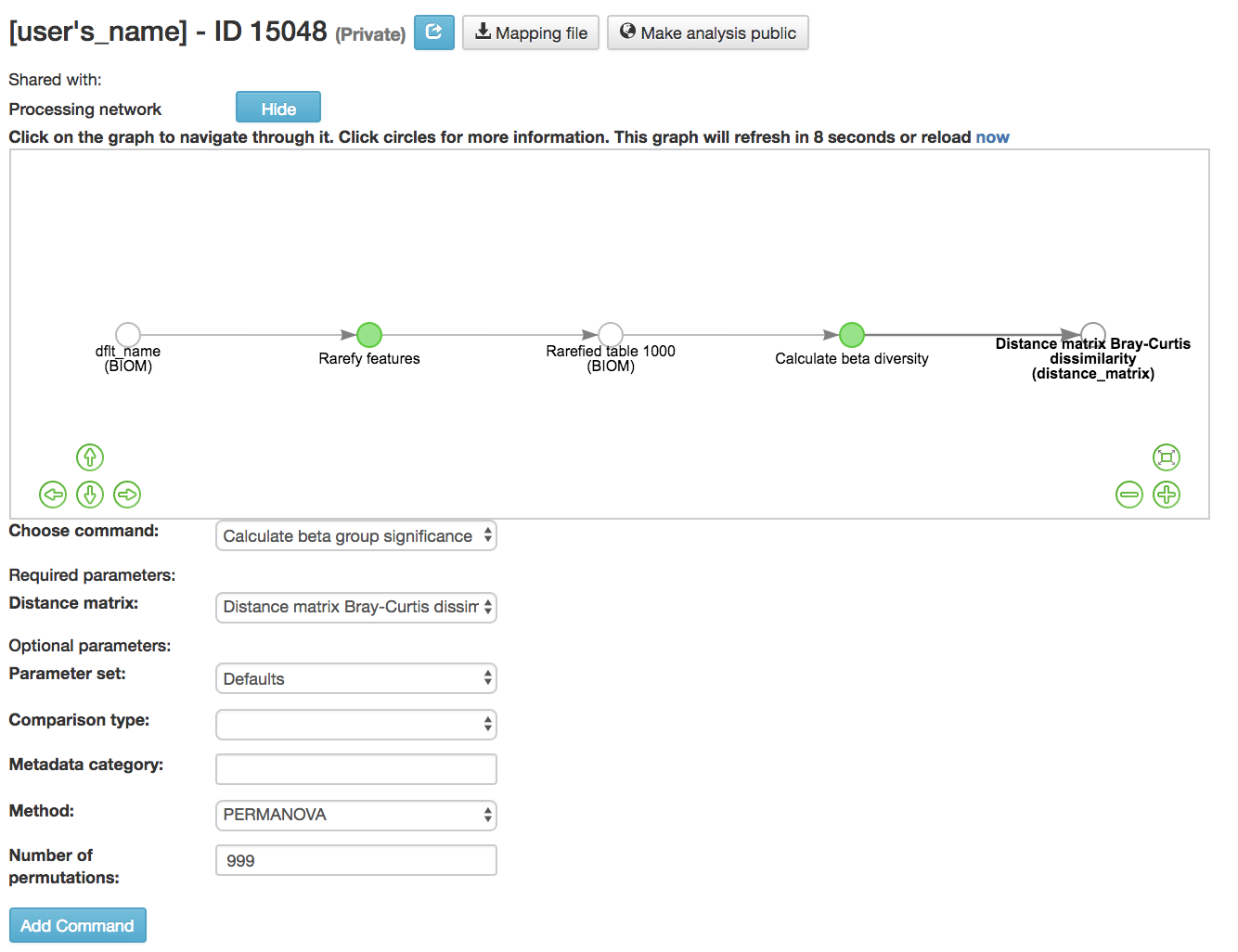
Calculate beta group significance: Determines whether groups of samples are significantly different from one another using a permutation-based statistical test
Distance matrix (required): Matrix of distances between pairs of samples
Comparison Type (required): Perform or not perform pairwise tests between all pairs of groups in addition to the test across all groups
Metadata category (required): Category from metadata file or artifact viewable as metadata
Method (required): Correlation test being applied
Anosim [59] : Describes the strength and significance that a category has in determining the distances between points and can accept either categorical or continuous variables in the metadata mapping file
Permanova [60] : Describes the strength and significance that a category has in determining the distances between points and can accept categorical variables
Number of permutations (required): Number of permutations to be run when computing p-values
Calculating Beta Correlation
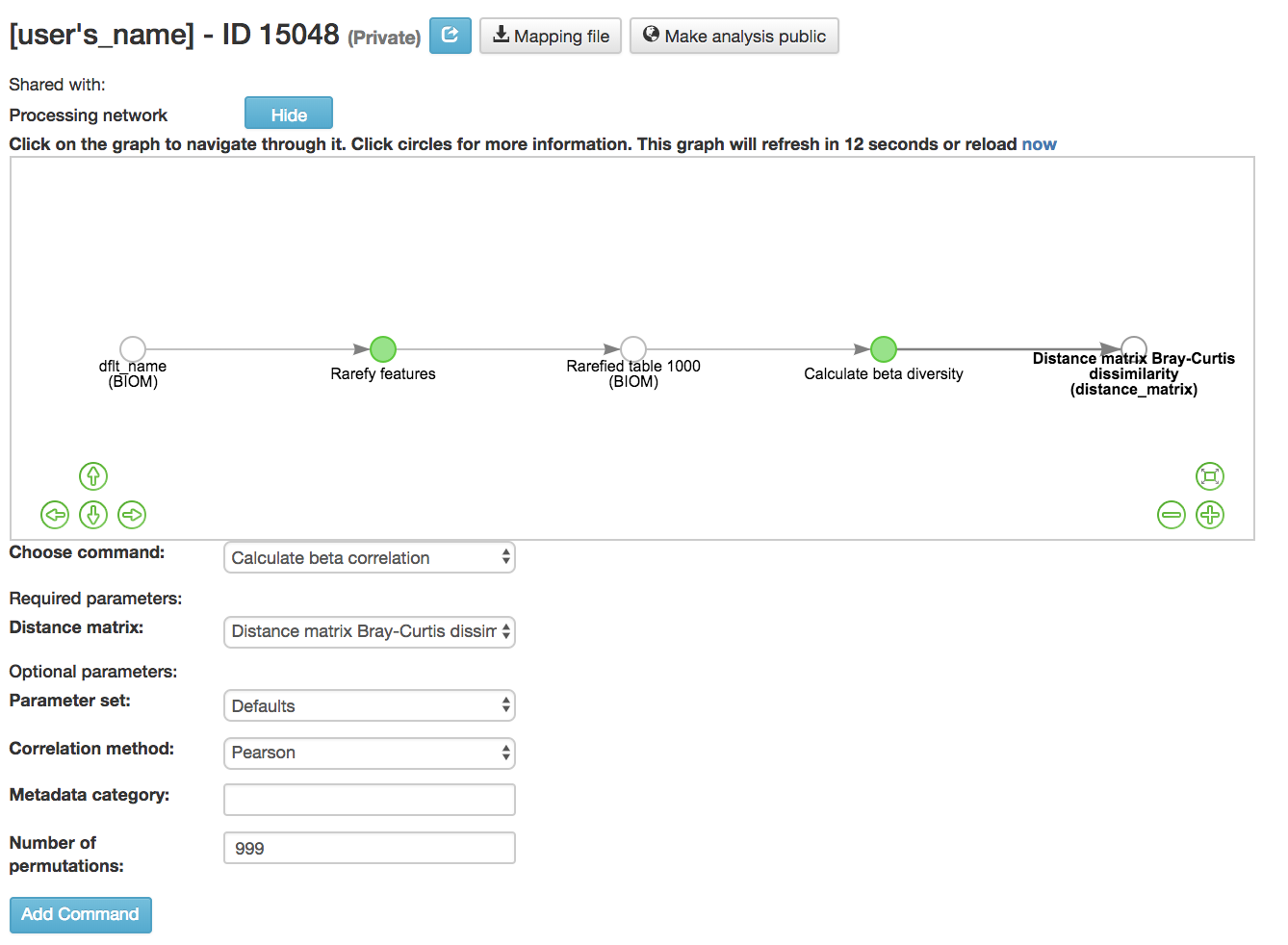
Calculate beta correlation: Identifies a correlation between the distance matrix and a numeric sample metadata category
Distance-matrix (required): Matrix of distances between pairs of samples
Correlation method (required): Correlation test being applied
Metadata-category (required): Category from metadata file or artifact viewable as metadata
Number of permutations (required): Number of permutations to be run when computing p-values
Processing Network Page: Results
Taxa Bar Plot
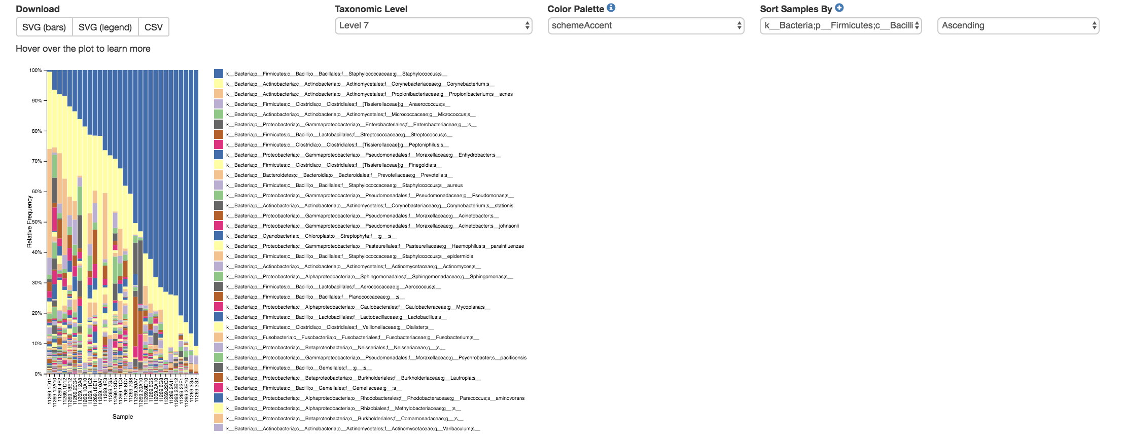
Taxonomic Level: How specific the taxa will be displayed
1- Kingdom, 2- Phylum, 3- Class, 4- Order, 5- Family, 6- Genus, 7- Species
Color Palette: Changes the coloring of your taxa bar plot
Discrete: Each taxon is a different color
Continuous: Each taxon is a different shade of one color
Sort Sample By: Sorts data by sample metadata or taxonomic abundance and either by ascending or descending order
Alpha Diversity Box Plots and Statistics
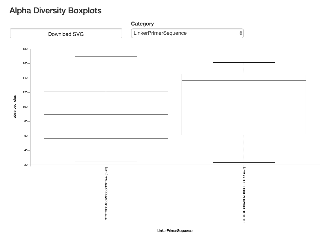
Boxplot: Shows how different measures of alpha diversity correlate with different metadata categories
Category: Choose the metadata category you would like to analyze
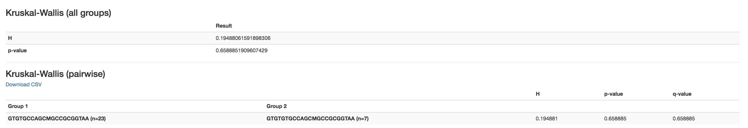
Kruskal-Wallis [61] : Result of Kruskal-Wallis tests
Says if the differences are statistically significant
Alpha Correlation Box Plots and Statistics
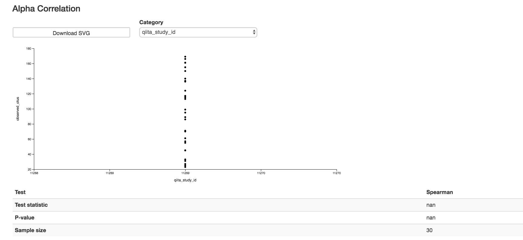
Boxplot: Shows how different measures of alpha diversity correlate with different metadata categories
Gives the Spearman or Pearson result (rho and p-value)
Beta Diversity Distance Matrix
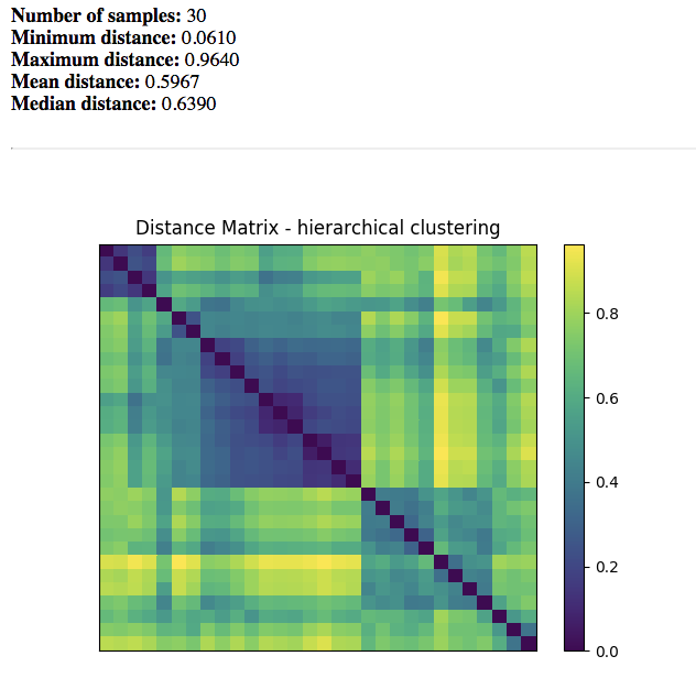
Distance Matrix: Dissimilarity value for each pairwise comparison
Principal Coordinate Analysis Plot
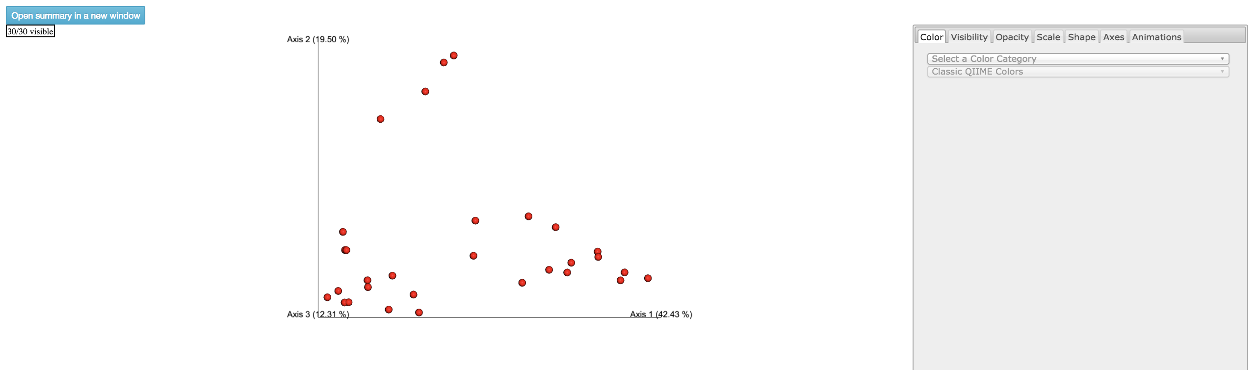
Emperor Plot: Visualization of similarities/dissimilarities between samples
Color: Choose colors for each group
Color Category: Groups each sample by the given category chosen by a given color
Visibility Allows for making certain samples invisible
Does not remove them from the analysis
Must perform filtering to do that
Opacity: Change the transparency of a given category
Scale: Change the size of a given category
Shape: Groups each sample by the given category chosen by a given shape
Axes: Change the position of the axis as well as the color of the graph
Animations: Traces the samples sorted by a metadata category
Requires a gradient column (the order in which samples are connected together, must be numeric) and a trajectory column (the way in which samples are grouped together) within the sample information file
Works best for time series
Beta Group Significance Box Plots and Statistics
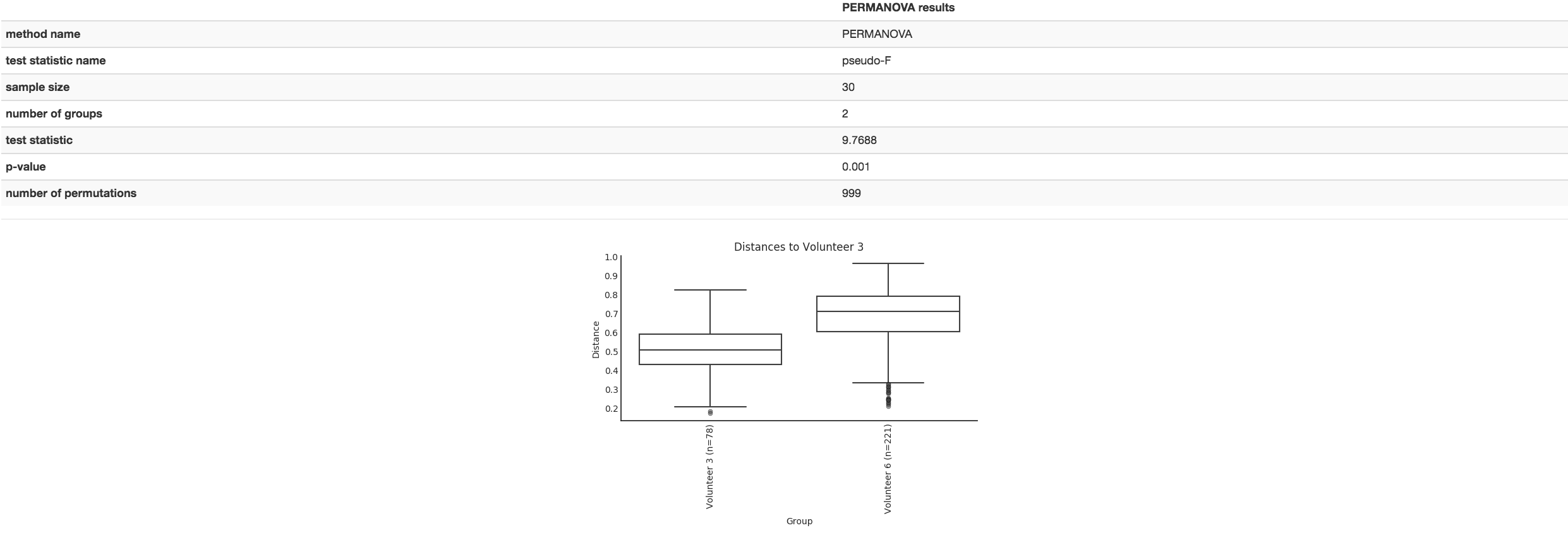
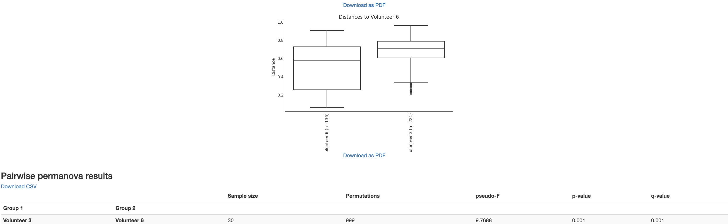
Boxplot: Shows how different measures of beta diversity correlate with different metadata categories
Gives the Permanova or Anosim result (psuedo-F and p-value)
Beta Correlation
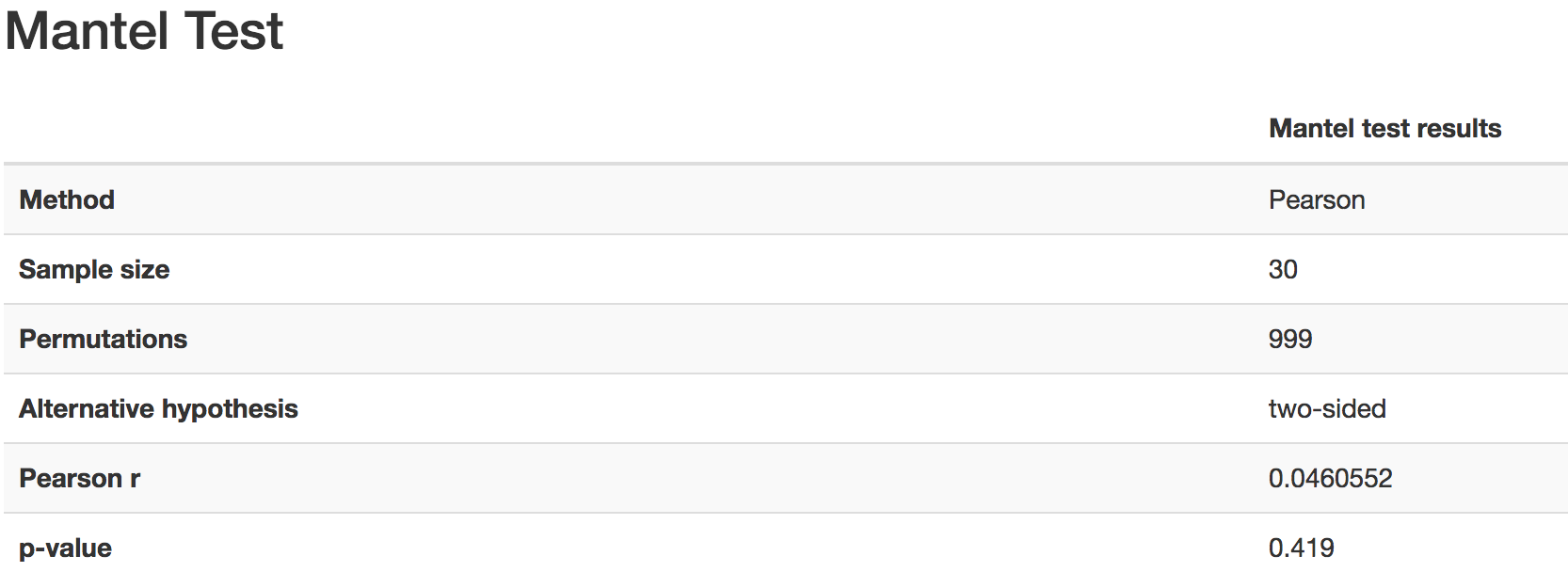
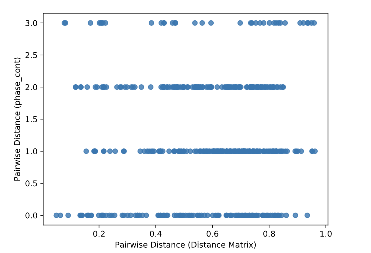
Gives the Spearman or Pearson result (rho and p-value)
Gives scatterplot of the distance matrix on the x-axis and the variable being tested on the y-axis